简单的PyTorch教程,来自官网教程60分钟PyTorch教程 、通过例子学PyTorch 和迁移学习教程 。
目录
60分钟PyTorch教程
什么是PyTorch?
Autograd: 自动求导
PyTorch神经网络简介
训练一个分类器
通过例子学PyTorch
迁移学习示例
60分钟PyTorch教程
什么是PyTorch?
PyTorch是一个基于Python的科学计算包,它主要有两个用途:
类似Numpy但是能利用GPU加速
一个非常灵活和快速的用于深度学习的研究平台
Tensor
Tensor类似与NumPy的ndarray,但是可以用GPU加速。使用前我们需要导入torch包:
1
2
from __future__ import print_function import torch
下面的代码构造一个5×35×3的未初始化的矩阵:
1
2
3
4
5
6
7
8
9
x = torch.empty(5, 3) print(x) # 输出: tensor([[-1.9998e+05, 4.5818e-41, 3.4318e-37], [ 0.0000e+00, 0.0000e+00, 0.0000e+00], [ 0.0000e+00, 0.0000e+00, 1.2877e+29], [ 2.0947e-30, 0.0000e+00, 0.0000e+00], [ 0.0000e+00, 0.0000e+00, -4.5328e+05]])
我们可以使用rand随机初始化一个矩阵:
1
2
3
4
5
6
7
8
9
x = torch.rand(5, 3) print(x) #输出: tensor([[ 0.9656, 0.5782, 0.0482], [ 0.7462, 0.5838, 0.1844], [ 0.8262, 0.4507, 0.6128], [ 0.2961, 0.8956, 0.3092], [ 0.4973, 0.2203, 0.9200]])
下面的代码构造一个用零初始化的矩阵,它的类型(dtype)是long:
1
2
3
4
5
6
7
8
9
x = torch.zeros(5, 3, dtype=torch.long) print(x) #输出: tensor([[ 0, 0, 0], [ 0, 0, 0], [ 0, 0, 0], [ 0, 0, 0], [ 0, 0, 0]])
我们也可以使用Python的数组来构造Tensor:
1
2
x = torch.tensor([5.5, 3]) print(x)
我们可以从已有的tensor信息(size和dtype)来构造tensor。但也可以用不同的dtype来构造。
1
2
3
4
5
x = x.new_ones(5, 3, dtype=torch.double) # new_* methods take in sizes print(x) x = torch.randn_like(x, dtype=torch.float) # override dtype! print(x)
我们可以是用size函数来看它的shape:
1
2
3
print(x.size()) #输出: torch.Size([5, 3])
注意torch.Size其实是一个tuple,因此它支持所有的tuple操作。
Operation
接下来我们来学习一些PyTorch的Operation。Operation一般可以使用函数的方式使用,但是为了方便使用,PyTorch重载了一些常见的运算符,因此我们可以这样来进行Tensor的加法:
1
2
y = torch.rand(5, 3) print(x + y)
我们也可以用add函数来实现加法:
我们也可以给加法提供返回值(而不是生成一个新的返回值):
1
2
3
result = torch.empty(5, 3) torch.add(x, y, out=result) # x + y的结果放到result里。 print(result)
我们也可以把相加的结果直接修改第一个被加数:
1
2
3
# 把x加到y y.add_(x) print(y)
注意:就地修改tensor的operation以下划线结尾。比如: x.copy_(y), x.t_(), 都会修改x。
Tensor的变换
我们也可以使用类似numpy的下标运算来操作PyTorch的Tensor:
如果想resize或者reshape一个Tensor,我们可以使用torch.view:
1 2 3 4 x = torch.randn(4, 4) y = x.view(16) z = x.view(-1, 8) # -1的意思是让PyTorch自己推断出第一维的大小。 print(x.size(), y.size(), z.size())
如果一个tensor只有一个元素,可以使用item()函数来把它变成一个Python number:
1 2 3 4 5 6 7 8 x = torch.randn(1) print(x) #输出的是一个Tensor tensor([-0.6966]) print(x.item()) #输出的是一个数 -0.6966081857681274
Tensor与Numpy的互相转换
Torch Tensor和NumPy数组的转换非常容易。它们会共享内存地址,因此修改一方会影响另一方。把一个Torch Tensor转换成NumPy数组的代码示例为:
1 2 3 4 5 6 a = torch.ones(5) print(a) #tensor([ 1., 1., 1., 1., 1.]) b = a.numpy() print(b) #[1. 1. 1. 1. 1.]
修改一个会影响另外一个:
1 2 3 4 5 a.add_(1) print(a) # tensor([ 2., 2., 2., 2., 2.]) print(b) # [2. 2. 2. 2. 2.]
把把NumPy数组转成Torch Tensor的代码示例为:
1 2 3 4 5 6 7 8 import numpy as np a = np.ones(5) b = torch.from_numpy(a) np.add(a, 1, out=a) print(a) # [2. 2. 2. 2. 2.] print(b) # tensor([ 2., 2., 2., 2., 2.], dtype=torch.float64)
CPU上的所有类型的Tensor(除了CharTensor)都可以和Numpy数组来回转换。
CUDA Tensor
Tensor可以使用to()方法来移到任意设备上:
1 2 3 4 5 6 7 8 9 10 11 12 13 # 如果有CUDA # 我们会使用``torch.device``来把tensors放到GPU上 if torch.cuda.is_available(): device = torch.device("cuda") # 一个CUDA device对象。 y = torch.ones_like(x, device=device) # 直接在GPU上创建tensor x = x.to(device) # 也可以使用``.to("cuda")``把一个tensor从CPU移到GPU上 z = x + y print(z) print(z.to("cpu", torch.double)) # ``.to``也可以在移动的过程中修改dtype # 输出: tensor([ 0.3034], device='cuda:0') tensor([ 0.3034], dtype=torch.float64)
Autograd: 自动求导
PyTorch的核心是autograd包。 我们首先简单的了解一些,然后用PyTorch开始训练第一个神经网络。autograd为所有用于Tensor的operation提供自动求导的功能。我们通过一些简单的例子来学习它基本用法。
从自动求导看Tensor
torch.Tensor 是这个包的核心类。如果它的属性requires_grad是True,那么PyTorch就会追踪所有与之相关的operation。当完成(正向)计算之后, 我们可以调用backward(),PyTorch会自动的把所有的梯度都计算好。与这个tensor相关的梯度都会累加到它的grad属性里。
如果不想计算这个tensor的梯度,我们可以调用detach(),这样它就不会参与梯度的计算了。为了阻止PyTorch记录用于梯度计算相关的信息(从而节约内存),我们可以使用 with torch.no_grad()。这在模型的预测时非常有用,因为预测的时候我们不需要计算梯度,否则我们就得一个个的修改Tensor的requires_grad属性,这会非常麻烦。
关于autograd的实现还有一个很重要的Function类。Tensor和Function相互连接从而形成一个有向无环图, 这个图记录了计算的完整历史。每个tensor有一个grad_fn属性来引用创建这个tensor的Function(用户直接创建的Tensor,这些Tensor的grad_fn是None)。
如果你想计算梯度,可以对一个Tensor调用它的backward()方法。如果这个Tensor是一个scalar(只有一个数),那么调用时不需要传任何参数。如果Tensor多于一个数,那么需要传入和它的shape一样的参数,表示反向传播过来的梯度。
创建tensor时设置属性requires_grad=True,PyTorch就会记录用于反向梯度计算的信息:
1 2 x = torch.ones(2, 2, requires_grad=True) print(x)
然后我们通过operation产生新的tensor:
是通过operation产生的tensor,因此它的grad_fn不是None。
1 2 print(y.grad_fn) # <AddBackward0 object at 0x7f35409a68d0>
再通过y得到z和out
1 2 3 4 5 6 z = y * y * 3 out = z.mean() print(z, out) # z = tensor([[ 27., 27.],[ 27., 27.]]) # out = tensor(27.)
requires_grad_()函数会修改一个Tensor的requires_grad。
1 2 3 4 5 6 7 a = torch.randn(2, 2) a = ((a * 3) / (a - 1)) print(a.requires_grad) a.requires_grad_(True) print(a.requires_grad) b = (a * a).sum() print(b.grad_fn)
输出是:
1 2 3 False True <SumBackward0 object at 0x7f35766827f0>
梯度
现在我们里反向计算梯度。因为out是一个scalar,因此out.backward()等价于out.backward(torch.tensor(1))。
我们可以打印梯度d(out)/dx:
1 2 3 print(x.grad) # tensor([[ 4.5000, 4.5000], [ 4.5000, 4.5000]])
我们手动计算来验证一下。为了简单,我们把out记为o。 o=14∑izio=14∑izi, zi=3(xi+2)2zi=3(xi+2)2 并且 zi∣∣xi=1=27zi|xi=1=27。
因此,∂o∂xi=32(xi+2)∂o∂xi=32(xi+2),因此∂o∂xi∣∣xi=1=92=4.5∂o∂xi|xi=1=92=4.5。
我们也可以用autograd做一些很奇怪的事情!比如y和x的关系是while循环的关系(似乎很难用一个函数直接表示y和x的关系?对x不断平方直到超过1000,这是什么函数?)
1 2 3 4 5 6 7 8 9 10 11 12 13 x = torch.randn(3, requires_grad=True) y = x * 2 while y.data.norm() < 1000: y = y * 2 print(y) # tensor([ -692.4808, 1686.1211, 667.7313]) gradients = torch.tensor([0.1, 1.0, 0.0001], dtype=torch.float) y.backward(gradients) print(x.grad) # tensor([ 102.4000, 1024.0000, 0.1024])
我们可以使用”with torch.no_grad()”来停止梯度的计算:
1 2 3 4 5 print(x.requires_grad) print((x ** 2).requires_grad) with torch.no_grad(): print((x ** 2).requires_grad)
输出为:
PyTorch神经网络简介
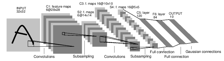
神经网络可以通过torch.nn包来创建。我们之前简单的了解了autograd,而nn会使用autograd来定义模型以及求梯度。一个nn.Module对象包括了许多网络层(layer),并且有一个forward(input)方法来返回output。如下图所示,我们会定义一个卷积网络来识别mnist图片。
训练一个神经网络通常需要如下步骤:
定义网络
1 2 3 4 5 6 7 8 9 10 11 12 13 14 15 16 17 18 19 20 21 22 23 24 25 26 27 28 29 30 31 32 33 34 35 36 37 38 39 40 41 42 43 44 45 46 import torch import torch.nn as nn import torch.nn.functional as F class Net(nn.Module): def __init__(self): super(Net, self).__init__() # 输入是1个通道的灰度图,输出6个通道(feature map),使用5x5的卷积核 self.conv1 = nn.Conv2d(1, 6, 5) # 第二个卷积层也是5x5,有16个通道 self.conv2 = nn.Conv2d(6, 16, 5) # 全连接层 self.fc1 = nn.Linear(16 * 5 * 5, 120) self.fc2 = nn.Linear(120, 84) self.fc3 = nn.Linear(84, 10) def forward(self, x): # 32x32 -> 28x28 -> 14x14 x = F.max_pool2d(F.relu(self.conv1(x)), (2, 2)) # 14x14 -> 10x10 -> 5x5 x = F.max_pool2d(F.relu(self.conv2(x)), 2) x = x.view(-1, self.num_flat_features(x)) x = F.relu(self.fc1(x)) x = F.relu(self.fc2(x)) x = self.fc3(x) return x def num_flat_features(self, x): size = x.size()[1:] # 除了batch维度之外的其它维度。 num_features = 1 for s in size: num_features *= s return num_features net = Net() print(net) # Net( (conv1): Conv2d(1, 6, kernel_size=(5, 5), stride=(1, 1)) (conv2): Conv2d(6, 16, kernel_size=(5, 5), stride=(1, 1)) (fc1): Linear(in_features=400, out_features=120, bias=True) (fc2): Linear(in_features=120, out_features=84, bias=True) (fc3): Linear(in_features=84, out_features=10, bias=True) )
我们只需要定义forward函数,而backward函数会自动通过autograd创建。在forward函数里可以使用任何处理Tensor的函数。我们可以使用函数net.parameters()来得到模型所有的参数。
1 2 3 4 5 params = list(net.parameters()) print(len(params)) # 10 print(params[0].size()) # conv1的weight # torch.Size([6, 1, 5, 5])
测试网络
接着我们尝试一个随机的32x32的输入来检验(sanity check)网络定义没有问题。注意:这个网络(LeNet)期望的输入大小是32x32。如果使用MNIST数据集(28x28),我们需要缩放到32x32。
1 2 3 4 5 input = torch.randn(1, 1, 32, 32) out = net(input) print(out) # tensor([[-0.0198, 0.0438, 0.0930, -0.0267, -0.0344, 0.0330, 0.0664, 0.1244, -0.0379, 0.0890]])
默认的梯度会累加,因此我们通常在backward之前清除掉之前的梯度值:
1 2 net.zero_grad() out.backward(torch.randn(1, 10))
注意:torch.nn只支持mini-batches的输入。整个torch.nn包的输入都必须第一维是batch,即使只有一个样本也要弄成batch是1的输入。
比如,nn.Conv2d的输入是一个4D的Tensor,shape是nSamples x nChannels x Height x Width。如果你只有一个样本(nChannels x Height x Width),那么可以使用input.unsqueeze(0)来增加一个batch维。
损失函数
损失函数的参数是(output, target)对,output是模型的预测,target是实际的值。损失函数会计算预测值和真实值的差别,损失越小说明预测的越准。
PyTorch提供了这里有许多不同的损失函数: http://pytorch.org/docs/nn.html#loss-functions。最简单的一个损失函数是:nn.MSELoss,它会计算预测值和真实值的均方误差。比如:
1 2 3 4 5 6 7 output = net(input) target = torch.arange(1, 11) # 随便伪造的一个“真实值” target = target.view(1, -1) # 把它变成output的shape(1, 10) criterion = nn.MSELoss() loss = criterion(output, target) print(loss)
如果从loss往回走,需要使用tensor的grad_fn属性,我们Negative看到这样的计算图:
1 2 3 4 input -> conv2d -> relu -> maxpool2d -> conv2d -> relu -> maxpool2d -> view -> linear -> relu -> linear -> relu -> linear -> MSELoss -> loss
因此当调用loss.backward()时,PyTorch会计算这个图中所有requires_grad=True的tensor关于loss的梯度。
1 2 3 4 5 6 7 8 print(loss.grad_fn) # MSELoss print(loss.grad_fn.next_functions[0][0]) # Add print(loss.grad_fn.next_functions[0][0].next_functions[0][0]) # Expand #输出: <MseLossBackward object at 0x7f445b3a2dd8> <AddmmBackward object at 0x7f445b3a2eb8> <ExpandBackward object at 0x7f445b3a2dd8>
计算梯度
在调用loss.backward()之前,我们需要清除掉tensor里之前的梯度,否则会累加进去。
1 2 3 4 5 6 7 8 9 net.zero_grad() # 清掉tensor里缓存的梯度值。 print('conv1.bias.grad before backward') print(net.conv1.bias.grad) loss.backward() print('conv1.bias.grad after backward') print(net.conv1.bias.grad)
更新参数
更新参数最简单的方法是使用随机梯度下降(SGD): weight=weight−learningrate∗gradientweight=weight−learningrate∗gradient 我们可以使用如下简单的代码来实现更新:
1 2 3 learning_rate = 0.01 for f in net.parameters(): f.data.sub_(f.grad.data * learning_rate)
通常我们会使用更加复杂的优化方法,比如SGD, Nesterov-SGD, Adam, RMSProp等等。为了实现这些算法,我们可以使用torch.optim包,它的用法也非常简单:
1 2 3 4 5 6 7 8 9 10 11 import torch.optim as optim # 创建optimizer,需要传入参数和learning rate optimizer = optim.SGD(net.parameters(), lr=0.01) # 清除梯度 optimizer.zero_grad() output = net(input) loss = criterion(output, target) loss.backward() optimizer.step() # optimizer会自动帮我们更新参数
注意:即使使用optimizer,我们也需要清零梯度。但是我们不需要一个个的清除,而是用optimizer.zero_grad()一次清除所有。
训练一个分类器
介绍了PyTorch神经网络相关包之后我们就可以用这些知识来构建一个分类器了。
如何进行数据处理
一般地,当我们处理图片、文本、音频或者视频数据的时候,我们可以使用python代码来把它转换成numpy数组。然后再把numpy数组转换成torch.xxxTensor。
对于处理图像,常见的lib包括Pillow和OpenCV
对于音频,常见的lib包括scipy和librosa
对于文本,可以使用标准的Python库,另外比较流行的lib包括NLTK和SpaCy
对于视觉问题,PyTorch提供了一个torchvision包(需要单独安装),它对于常见数据集比如Imagenet, CIFAR10, MNIST等提供了加载的方法。并且它也提供很多数据变化的工具,包括torchvision.datasets和torch.utils.data.DataLoader。这会极大的简化我们的工作,避免重复的代码。
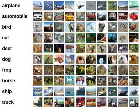
在这个教程里,我们使用CIFAR10数据集。它包括十个类别:”airplane”, “automobile”, “bird”, “cat”, “deer”, “dog”, “frog”, “horse”, “ship”,”truck”。图像的对象是3x32x32,也就是3通道(RGB)的32x32的图片。下面是一些样例图片。
训练的步骤
使用torchvision加载和预处理CIFAR10训练和测试数据集。
定义卷积网络
定义损失函数
用训练数据训练模型
用测试数据测试模型
数据处理
通过使用torchvision,我们可以轻松的加载CIFAR10数据集。首先我们导入相关的包:
1 2 3 import torch import torchvision import torchvision.transforms as transforms
torchvision读取的datasets是PILImage对象,它的取值范围是[0, 1],我们把它转换到范围[-1, 1]。
1 2 3 4 5 6 7 8 9 10 11 12 13 14 15 16 transform = transforms.Compose( [transforms.ToTensor(), transforms.Normalize((0.5, 0.5, 0.5), (0.5, 0.5, 0.5))]) trainset = torchvision.datasets.CIFAR10(root='/path/to/data', train=True, download=True, transform=transform) trainloader = torch.utils.data.DataLoader(trainset, batch_size=4, shuffle=True, num_workers=2) testset = torchvision.datasets.CIFAR10(root='/path/to/data', train=False, download=True, transform=transform) testloader = torch.utils.data.DataLoader(testset, batch_size=4, shuffle=False, num_workers=2) classes = ('plane', 'car', 'bird', 'cat', 'deer', 'dog', 'frog', 'horse', 'ship', 'truck')
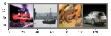
我们来看几张图片,如下图 所示,显示图片的代码如下:
1 2 3 4 5 6 7 8 9 10 11 12 13 14 15 16 17 18 19 20 import matplotlib.pyplot as plt import numpy as np # 显示图片的函数 def imshow(img): img = img / 2 + 0.5 # [-1,1] -> [0,1] npimg = img.numpy() plt.imshow(np.transpose(npimg, (1, 2, 0))) # (channel, width, height) -> (width, height, channel) # 随机选择一些图片 dataiter = iter(trainloader) images, labels = dataiter.next() # 显示图片 imshow(torchvision.utils.make_grid(images)) # 打印label print(' '.join('%5s' % classes[labels[j]] for j in range(4)))
定义卷积网络
网络结构和上一节的介绍类似,只是输入通道从1变成3。
1 2 3 4 5 6 7 8 9 10 11 12 13 14 15 16 17 18 19 20 21 22 23 24 import torch.nn as nn import torch.nn.functional as F class Net(nn.Module): def __init__(self): super(Net, self).__init__() self.conv1 = nn.Conv2d(3, 6, 5) self.pool = nn.MaxPool2d(2, 2) self.conv2 = nn.Conv2d(6, 16, 5) self.fc1 = nn.Linear(16 * 5 * 5, 120) self.fc2 = nn.Linear(120, 84) self.fc3 = nn.Linear(84, 10) def forward(self, x): x = self.pool(F.relu(self.conv1(x))) x = self.pool(F.relu(self.conv2(x))) x = x.view(-1, 16 * 5 * 5) x = F.relu(self.fc1(x)) x = F.relu(self.fc2(x)) x = self.fc3(x) return x net = Net()
我们这里使用交叉熵损失函数,Optimizer使用带冲量的SGD。
1 2 3 4 import torch.optim as optim criterion = nn.CrossEntropyLoss() optimizer = optim.SGD(net.parameters(), lr=0.001, momentum=0.9)
我们遍历DataLoader进行训练。
1 2 3 4 5 6 7 8 9 10 11 12 13 14 15 16 17 18 19 20 21 22 23 24 for epoch in range(2): # 这里只迭代2个epoch,实际应该进行更多次训练 running_loss = 0.0 for i, data in enumerate(trainloader, 0): # 得到输入 inputs, labels = data # 梯度清零 optimizer.zero_grad() # forward + backward + optimize outputs = net(inputs) loss = criterion(outputs, labels) loss.backward() optimizer.step() # 定义统计信息 running_loss += loss.item() if i % 2000 == 1999: print('[%d, %5d] loss: %.3f' % (epoch + 1, i + 1, running_loss / 2000)) running_loss = 0.0 print('Finished Training')
在测试数据集上进行测试
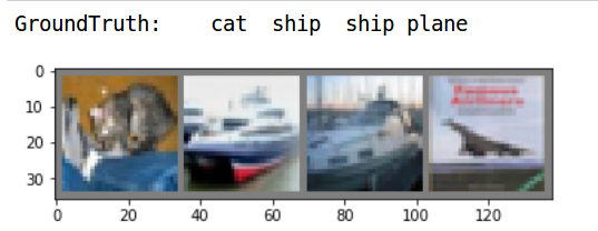
我们进行了2轮迭代,可以使用测试数据集上的数据来进行测试。首先我们随机抽取几个样本来进行测试。
1 2 3 4 5 6 dataiter = iter(testloader) images, labels = dataiter.next() imshow(torchvision.utils.make_grid(images)) print('GroundTruth: ', ' '.join('%5s' % classes[labels[j]] for j in range(4)))
随机选择出来的测试样例如下图所示。
我们用模型来预测一下,看看是否正确预测:
outputs是10个分类的logits。我们在训练的时候需要用softmax把它变成概率(CrossEntropyLoss帮我们做了),但是预测的时候没有必要,因为我们只需要知道哪个分类的概率大就行。
1 2 3 4 5 6 _, predicted = torch.max(outputs, 1) print('Predicted: ', ' '.join('%5s' % classes[predicted[j]] for j in range(4))) # cat ship ship ship
预测中的四个错了一个,似乎还不错。接下来我们看看在整个测试集合上的效果:
1 2 3 4 5 6 7 8 9 10 11 12 13 14 correct = 0 total = 0 with torch.no_grad(): for data in testloader: images, labels = data outputs = net(images) _, predicted = torch.max(outputs.data, 1) total += labels.size(0) correct += (predicted == labels).sum().item() print('Accuracy of the network on the 10000 test images: %d %%' % ( 100 * correct / total)) # Accuracy of the network on the 10000 test images: 55 %
看起来比随机的瞎猜要好,因为随机猜的准确率大概是10%的准确率,所以模型确实学到了一些东西。我们也可以看每个分类的准确率:
1 2 3 4 5 6 7 8 9 10 11 12 13 14 15 16 17 class_correct = list(0. for i in range(10)) class_total = list(0. for i in range(10)) with torch.no_grad(): for data in testloader: images, labels = data outputs = net(images) _, predicted = torch.max(outputs, 1) c = (predicted == labels).squeeze() for i in range(4): label = labels[i] class_correct[label] += c[i].item() class_total[label] += 1 for i in range(10): print('Accuracy of %5s : %2d %%' % ( classes[i], 100 * class_correct[i] / class_total[i]))
结果为:
1 2 3 4 5 6 7 8 9 10 Accuracy of plane : 52 % Accuracy of car : 66 % Accuracy of bird : 49 % Accuracy of cat : 34 % Accuracy of deer : 30 % Accuracy of dog : 45 % Accuracy of frog : 72 % Accuracy of horse : 71 % Accuracy of ship : 76 % Accuracy of truck : 55 %
GPU上训练
为了在GPU上训练,我们需要把Tensor移到GPU上。首先我们看看是否有GPU,如果没有,那么我们还是fallback到CPU。
1 2 3 device = torch.device("cuda:0" if torch.cuda.is_available() else "cpu") print(device) # cuda:0
用GPU进行训练:
1 2 3 4 5 6 7 8 9 10 11 12 13 14 15 16 17 18 19 20 21 22 23 24 25 26 27 28 29 30 31 32 33 34 35 36 37 38 39 40 41 42 43 44 45 46 47 48 class Net2(nn.Module): def __init__(self): super(Net2, self).__init__() self.conv1 = nn.Conv2d(3, 6, 5).to(device) self.pool = nn.MaxPool2d(2, 2).to(device) self.conv2 = nn.Conv2d(6, 16, 5).to(device) self.fc1 = nn.Linear(16 * 5 * 5, 120).to(device) self.fc2 = nn.Linear(120, 84).to(device) self.fc3 = nn.Linear(84, 10).to(device) def forward(self, x): x = self.pool(F.relu(self.conv1(x))) x = self.pool(F.relu(self.conv2(x))) x = x.view(-1, 16 * 5 * 5) x = F.relu(self.fc1(x)) x = F.relu(self.fc2(x)) x = self.fc3(x) return x net = Net2() criterion = nn.CrossEntropyLoss() optimizer = optim.SGD(net.parameters(), lr=0.001, momentum=0.9) for epoch in range(20): running_loss = 0.0 for i, data in enumerate(trainloader, 0): # 得到输入 inputs, labels = data inputs, labels = inputs.to(device), labels.to(device) # 梯度清零 optimizer.zero_grad() # forward + backward + optimize outputs = net(inputs) loss = criterion(outputs, labels) loss.backward() optimizer.step() # 定义统计信息 running_loss += loss.item() if i % 2000 == 1999: print('[%d, %5d] loss: %.3f' % (epoch + 1, i + 1, running_loss / 2000)) running_loss = 0.0 print('Finished Training')
通过例子学PyTorch
下面我们通过使用不同的方法来实现一个简单的三层(一个隐层)的全连接神经网络来熟悉PyTorch的常见用法。
使用Numpy实现三层神经网络
我们需要实现一个全连接的激活为ReLU的网络,它只有一个隐层,没有bias,用于回归预测一个值,loss是计算实际值和预测值的欧氏距离。这里完全使用numpy手动的进行前向和后向计算。numpy数组就是一个n维的数值,它并不知道任何关于深度学习、梯度下降或者计算图的东西,它只是进行数值运算。
1 2 3 4 5 6 7 8 9 10 11 12 13 14 15 16 17 18 19 20 21 22 23 24 25 26 27 28 29 30 31 32 33 34 35 36 import numpy as np # N是batch size;D_in是输入大小 # H是隐层的大小;D_out是输出大小。 N, D_in, H, D_out = 64, 1000, 100, 10 # 随机产生输入与输出 x = np.random.randn(N, D_in) y = np.random.randn(N, D_out) # 随机初始化参数 w1 = np.random.randn(D_in, H) w2 = np.random.randn(H, D_out) learning_rate = 1e-6 for t in range(500): # 前向计算y h = x.dot(w1) h_relu = np.maximum(h, 0) y_pred = h_relu.dot(w2) # 计算loss loss = np.square(y_pred - y).sum() print(t, loss) # 反向计算梯度 grad_y_pred = 2.0 * (y_pred - y) grad_w2 = h_relu.T.dot(grad_y_pred) grad_h_relu = grad_y_pred.dot(w2.T) grad_h = grad_h_relu.copy() grad_h[h < 0] = 0 grad_w1 = x.T.dot(grad_h) # 更新参数 w1 -= learning_rate * grad_w1 w2 -= learning_rate * grad_w2
使用Tensor来实现三层神经网络
和前面一样,我们还是实现一个全连接的Relu激活的网络,它只有一个隐层并且没有bias。loss是预测与真实值的欧氏距离。之前我们用Numpy实现,自己手动前向计算loss,反向计算梯度。这里还是一样,只不过把numpy数组换成了PyTorch的Tensor。但是使用PyTorch的好处是我们可以利用GPU来加速计算,如果想用GPU计算,我们值需要在创建tensor的时候指定device为gpu。
1 2 3 4 5 6 7 8 9 10 11 12 13 14 15 16 17 18 19 20 21 22 23 24 25 26 27 28 29 30 31 32 33 import torch dtype = torch.float device = torch.device("cpu") # device = torch.device("cuda:0") # 如果想在GPU上运算,把这行注释掉。 N, D_in, H, D_out = 64, 1000, 100, 10 x = torch.randn(N, D_in, device=device, dtype=dtype) y = torch.randn(N, D_out, device=device, dtype=dtype) w1 = torch.randn(D_in, H, device=device, dtype=dtype) w2 = torch.randn(H, D_out, device=device, dtype=dtype) learning_rate = 1e-6 for t in range(500): h = x.mm(w1) h_relu = h.clamp(min=0) # 使用clamp(min=0)来实现ReLU y_pred = h_relu.mm(w2) loss = (y_pred - y).pow(2).sum().item() print(t, loss) grad_y_pred = 2.0 * (y_pred - y) grad_w2 = h_relu.t().mm(grad_y_pred) grad_h_relu = grad_y_pred.mm(w2.t()) grad_h = grad_h_relu.clone() grad_h[h < 0] = 0 grad_w1 = x.t().mm(grad_h) w1 -= learning_rate * grad_w1 w2 -= learning_rate * grad_w2
实现autograd来实现三层神经网络
还是和前面一样实现一个全连接的网络,只有一个隐层而且没有bias,使用欧氏距离作为损失函数。这个实现使用PyTorch的Tensor来计算前向阶段,然后使用PyTorch的autograd来自动帮我们反向计算梯度。PyTorch的Tensor代表了计算图中的一个节点。如果x是一个Tensor并且x.requires_grad=True,那么x.grad这个Tensor会保存某个scalar(通常是loss)对x的梯度。
1 2 3 4 5 6 7 8 9 10 11 12 13 14 15 16 17 18 19 20 21 22 23 24 25 26 27 28 29 30 31 32 33 34 35 36 37 38 39 40 41 42 43 44 45 46 47 48 import torch dtype = torch.float device = torch.device("cpu") # device = torch.device("cuda:0") # 如果有GPU可以注释掉这行 # N是batch size;D_in是输入大小 # H是隐层的大小;D_out是输出大小。 N, D_in, H, D_out = 64, 1000, 100, 10 # 创建随机的Tensor作为输入和输出 # 输入和输出需要的requires_grad=False(默认), # 因为我们不需要计算loss对它们的梯度。 x = torch.randn(N, D_in, device=device, dtype=dtype) y = torch.randn(N, D_out, device=device, dtype=dtype) # 创建weight的Tensor,需要设置requires_grad=True w1 = torch.randn(D_in, H, device=device, dtype=dtype, requires_grad=True) w2 = torch.randn(H, D_out, device=device, dtype=dtype, requires_grad=True) learning_rate = 1e-6 for t in range(500): # Forward阶段: mm实现矩阵乘法,但是它不支持broadcasting。 # 如果需要broadcasting,可以使用matmul # clamp本来的用途是把值clamp到指定的范围,这里实现ReLU。 y_pred = x.mm(w1).clamp(min=0).mm(w2) # pow(2)实现平方计算。 # loss.item()得到这个tensor的值。也可以直接打印loss,这会打印很多附加信息。 loss = (y_pred - y).pow(2).sum() print(t, loss.item()) # 使用autograd进行反向计算。它会计算loss对所有对它有影响的 # requires_grad=True的Tensor的梯度。 loss.backward() # 手动使用梯度下降更新参数。一定要把更新的代码放到torch.no_grad()里 # 否则下面的更新也会计算梯度。后面我们会使用torch.optim.SGD, # 它会帮我们管理这些用于更新梯度的计算。 with torch.no_grad(): w1 -= learning_rate * w1.grad w2 -= learning_rate * w2.grad # 手动把梯度清零 w1.grad.zero_() w2.grad.zero_()
使用自定义的ReLU函数
这里还是那个全连接网络的例子,不过这里我们不使用clamp来实现ReLU,而是我们自己来实现一个MyReLU的函数。
1 2 3 4 5 6 7 8 9 10 11 12 13 14 15 16 17 18 19 20 21 22 23 24 25 26 27 28 29 30 31 32 33 34 35 36 37 38 39 40 41 42 43 44 45 46 47 48 49 50 51 52 53 54 55 56 57 58 59 60 61 62 import torch class MyReLU(torch.autograd.Function): """ 为了实现自定义的实现autograd的函数,我们需要基础torch.autograd.Function, 然后再实现forward和backward两个函数。 """ @staticmethod def forward(ctx, input): """ 在forward函数,我们的输入是input,然后我们根据input计算输出。 # 同时为了下面的backward, 我们需要使用save_for_backward来保存用于反向计算的数据到ctx里, # 这里我们需要保存input。 """ ctx.save_for_backward(input) return input.clamp(min=0) @staticmethod def backward(ctx, grad_output): """ 从ctx.saved_tensors里恢复input 然后用input计算梯度 """ input, = ctx.saved_tensors grad_input = grad_output.clone() grad_input[input < 0] = 0 return grad_input dtype = torch.float device = torch.device("cpu") N, D_in, H, D_out = 64, 1000, 100, 10 x = torch.randn(N, D_in, device=device, dtype=dtype) y = torch.randn(N, D_out, device=device, dtype=dtype) w1 = torch.randn(D_in, H, device=device, dtype=dtype, requires_grad=True) w2 = torch.randn(H, D_out, device=device, dtype=dtype, requires_grad=True) learning_rate = 1e-6 for t in range(500): # 为了调用我们自定义的函数,我们需要使用Function.apply方法,把它命名为'relu' relu = MyReLU.apply # 我们使用自定义的ReLU来进行Forward计算 y_pred = relu(x.mm(w1)).mm(w2) loss = (y_pred - y).pow(2).sum() print(t, loss.item()) loss.backward() with torch.no_grad(): w1 -= learning_rate * w1.grad w2 -= learning_rate * w2.grad w1.grad.zero_() w2.grad.zero_()
和Tensorflow的对比
这里我们还是和前面一样,实现一个隐层的全连接神经网络,优化的目标函数是预测值和真实值的欧氏距离。这个实现使用基本的Tensorflow操作来构建一个计算图,然后多次执行这个计算图来训练网络。Tensorflow和PyTorch最大的区别之一就是Tensorflow使用静态计算图和PyTorch使用动态计算图。在Tensorflow里,我们首先构建计算图,然后多次执行它。
1 2 3 4 5 6 7 8 9 10 11 12 13 14 15 16 17 18 19 20 21 22 23 24 25 26 27 28 29 30 31 32 33 34 35 36 37 38 39 40 41 42 43 44 45 46 47 48 49 50 51 52 53 54 55 56 57 import tensorflow as tf import numpy as np # 首先构建计算图。 # N是batch大小;D_in是输入大小。 # H是隐单元个数;D_out是输出大小。 N, D_in, H, D_out = 64, 1000, 100, 10 # 输入和输出是placeholder,在用session执行graph的时候 # 我们会feed进去一个batch的训练数据。 x = tf.placeholder(tf.float32, shape=(None, D_in)) y = tf.placeholder(tf.float32, shape=(None, D_out)) # 创建变量,并且随机初始化。 # 在Tensorflow里,变量的生命周期是整个session,因此适合用它来保存模型的参数。 w1 = tf.Variable(tf.random_normal((D_in, H))) w2 = tf.Variable(tf.random_normal((H, D_out))) # Forward pass:计算模型的预测值y_pred # 注意和PyTorch不同,这里不会执行任何计算, # 而只是定义了计算,后面用session.run的时候才会真正的执行计算。 h = tf.matmul(x, w1) h_relu = tf.maximum(h, tf.zeros(1)) y_pred = tf.matmul(h_relu, w2) # 计算loss loss = tf.reduce_sum((y - y_pred) ** 2.0) # 计算梯度。 grad_w1, grad_w2 = tf.gradients(loss, [w1, w2]) # 使用梯度下降来更新参数。assign同样也只是定义更新参数的操作,不会真正的执行。 # 在Tensorflow里,更新操作是计算图的一部分; # 而在PyTorch里,因为是动态的”实时“的计算, # 所以参数的更新只是普通的Tensor计算,不属于计算图的一部分。 learning_rate = 1e-6 new_w1 = w1.assign(w1 - learning_rate * grad_w1) new_w2 = w2.assign(w2 - learning_rate * grad_w2) # 计算图构建好了之后,我们需要创建一个session来执行计算图。 with tf.Session() as sess: # 首先需要用session初始化变量 sess.run(tf.global_variables_initializer()) # 这是fake的训练数据 x_value = np.random.randn(N, D_in) y_value = np.random.randn(N, D_out) for _ in range(500): # 用session多次的执行计算图。每次feed进去不同的数据。 # 这里是模拟的,实际应该每次feed一个batch的数据。 # run的第一个参数是需要执行的计算图的节点,它依赖的节点也会自动执行, # 因此我们不需要手动执行forward的计算。 # run返回这些节点执行后的值,并且返回的是numpy array loss_value, _, _ = sess.run([loss, new_w1, new_w2], feed_dict={x: x_value, y: y_value}) print(loss_value)
使用nn模块来实现三层神经网络
我们接下来使用nn模块来实现这个简单的全连接网络。前面我们通过用Tensor和Operation等low-level API来创建 动态的计算图,这里我们使用更简单的high-level API。
1 2 3 4 5 6 7 8 9 10 11 12 13 14 15 16 17 18 19 20 21 22 23 24 25 26 27 28 29 30 31 import torch print(torch.__version__) # N是batch size;D_in是输入大小 # H是隐层的大小;D_out是输出大小。 N, D_in, H, D_out = 64, 1000, 100, 10 # 创建随机的Tensor作为输入和输出 x = torch.randn(N, D_in) y = torch.randn(N, D_out) # 使用nn包来定义网络。nn.Sequential是一个包含其它模块(Module)的模块。 # 每个Linear模块使用线性函数来计算,它会内部创建需要的weight和bias。 model = torch.nn.Sequential( torch.nn.Linear(D_in, H), torch.nn.ReLU(), torch.nn.Linear(H, D_out), ) # 常见的损失函数在nn包里也有,不需要我们自己实现 loss_fn = torch.nn.MSELoss(size_average=False) learning_rate = 1e-4 for t in range(500): # 前向计算:通过x来计算y。Module对象会重写__call__函数, # 因此我们可以把它当成函数来调用。 y_pred = model(x) # 计算loss loss = loss_fn(y_pred, y) print(t, loss.item()) # 梯度清空,调用Sequential对象的zero_grad后所有里面的变量都会清零梯度 model.zero_grad() # 反向计算梯度。我们通过Module定义的变量都会计算梯度。 loss.backward() # 更新参数,所有的参数都在model.paramenters()里 with torch.no_grad(): for param in model.parameters(): param -= learning_rate * param.grad
使用optim包
前面我们使用nn模块时是自己来更新模型参数的,PyTorch也提供了optim包,我们可以使用里面的Optimizer来自动的更新模型参数。除了最基本的SGD算法,这个包也实现了常见的SGD+momentum, RMSProp, Adam等算法。
1 2 3 4 5 6 7 8 9 10 11 12 13 14 15 16 17 18 19 20 21 22 23 24 25 26 27 import torch N, D_in, H, D_out = 64, 1000, 100, 10 x = torch.randn(N, D_in) y = torch.randn(N, D_out) model = torch.nn.Sequential( torch.nn.Linear(D_in, H), torch.nn.ReLU(), torch.nn.Linear(H, D_out), ) loss_fn = torch.nn.MSELoss(size_average=False) # 使用Adam算法,需要提供模型的参数和learning rate learning_rate = 1e-4 optimizer = torch.optim.Adam(model.parameters(), lr=learning_rate) for t in range(500): y_pred = model(x) loss = loss_fn(y_pred, y) print(t, loss.item()) # 梯度清零,原来调用的是model.zero_grad,现在调用的是optimizer的zero_grad optimizer.zero_grad() loss.backward() # 调用optimizer.step实现参数更新 optimizer.step()
自定义nn模块
对于复杂的网络结构,我们可以通过基础Module了自定义nn模块。这样的好处是用一个类来同样管理,而且更容易复用代码。
1 2 3 4 5 6 7 8 9 10 11 12 13 14 15 16 17 18 19 20 21 22 23 24 25 26 27 28 29 30 31 32 33 34 35 import torch class TwoLayerNet(torch.nn.Module): def __init__(self, D_in, H, D_out): """ 在构造函数里,我们定义两个nn.Linear模块,把它们保存到self里。 """ super(TwoLayerNet, self).__init__() self.linear1 = torch.nn.Linear(D_in, H) self.linear2 = torch.nn.Linear(H, D_out) def forward(self, x): """ 在forward函数里,我们需要根据网络结构来实现前向计算。 通常我们会上定义的模块来计算。 """ h_relu = self.linear1(x).clamp(min=0) y_pred = self.linear2(h_relu) return y_pred N, D_in, H, D_out = 64, 1000, 100, 10 x = torch.randn(N, D_in) y = torch.randn(N, D_out) model = TwoLayerNet(D_in, H, D_out) criterion = torch.nn.MSELoss(size_average=False) optimizer = torch.optim.SGD(model.parameters(), lr=1e-4) for t in range(500): y_pred = model(x) loss = criterion(y_pred, y) print(t, loss.item()) optimizer.zero_grad() loss.backward() optimizer.step()
流程控制和参数共享
为了展示PyTorch的动态图的能力,我们这里会实现一个很奇怪模型:这个全连接的网络的隐层个数是个1到4之间的随机数,而且这些网络层的参数是共享的。
1 2 3 4 5 6 7 8 9 10 11 12 13 14 15 16 17 18 19 20 21 22 23 24 25 26 27 28 29 30 31 32 33 34 35 36 37 38 39 40 import random import torch class DynamicNet(torch.nn.Module): def __init__(self, D_in, H, D_out): """ 构造3个nn.Linear实例。 """ super(DynamicNet, self).__init__() self.input_linear = torch.nn.Linear(D_in, H) self.middle_linear = torch.nn.Linear(H, H) self.output_linear = torch.nn.Linear(H, D_out) def forward(self, x): # 输入和输出层是固定的,但是中间层的个数是随机的(0,1,2), # 并且中间层的参数是共享的。 # 因为每次计算的计算图是动态(实时)构造的, # 所以我们可以使用普通的Python流程控制代码比如for循环 # 来实现。读者可以尝试一下怎么用TensorFlow来实现。 # 另外一点就是一个Module可以多次使用,这样就 # 可以实现参数共享。 h_relu = self.input_linear(x).clamp(min=0) for _ in range(random.randint(0, 3)): h_relu = self.middle_linear(h_relu).clamp(min=0) y_pred = self.output_linear(h_relu) return y_pred N, D_in, H, D_out = 64, 1000, 100, 10 x = torch.randn(N, D_in) y = torch.randn(N, D_out) model = DynamicNet(D_in, H, D_out) criterion = torch.nn.MSELoss(size_average=False) optimizer = torch.optim.SGD(model.parameters(), lr=1e-4, momentum=0.9) for t in range(500): y_pred = model(x) loss = criterion(y_pred, y) print(t, loss.item()) optimizer.zero_grad() loss.backward() optimizer.step()
迁移学习示例
在这个教程里,我们会学习怎么使用迁移学习来训练模型。通常我们的训练数据量不会很大,很难达到像ImageNet那样上百万的标注数据集。我们可以使用迁移学习来解决训练数据不足的问题。迁移学习里,我们根据训练数据的多少通常可以采取如下方法:
训练数据很少
那么我们通常把一个pretraning的网络的大部分固定住,然后只是把最后一个全连接层换成新的(最后一层通常是不一样的,因为分类的数量不同),然后只训练这一层
训练数据较多
我们可以把pretraining的网络的前面一些层固定住,但后面的层不固定,把最后一层换新的,然后训练
训练数据很多
所有的pretraining的层都可以fine-tuning,只是用pretraining的参数作为初始化参数。
首先我们引入依赖:
1 2 3 4 5 6 7 8 9 10 11 12 13 14 15 from __future__ import print_function, division import torch import torch.nn as nn import torch.optim as optim from torch.optim import lr_scheduler import numpy as np import torchvision from torchvision import datasets, models, transforms import matplotlib.pyplot as plt import time import os import copy plt.ion()
加载数据
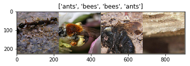
我们使用torchvision和torch.utils.data包来加载数据。我们要解决的问题是训练一个模型来区分蚂蚁和蜜蜂,每个类别我们大概有120个训练数据,另外每个类有75个验证数据。这是一个很小的训练集,如果直接用一个神经网络来训练,效果会很差。现在我们用迁移学习来解决这个问题。数据可以在这里 下载,下载后请解压到data目录下。
1 2 3 4 5 6 7 8 9 10 11 12 13 14 15 16 17 18 19 20 21 22 23 24 25 26 27 28 # 训练的时候会做数据增强和归一化 # 而验证的时候只做归一化 data_transforms = { 'train': transforms.Compose([ transforms.RandomResizedCrop(224), transforms.RandomHorizontalFlip(), transforms.ToTensor(), transforms.Normalize([0.485, 0.456, 0.406], [0.229, 0.224, 0.225]) ]), 'val': transforms.Compose([ transforms.Resize(256), transforms.CenterCrop(224), transforms.ToTensor(), transforms.Normalize([0.485, 0.456, 0.406], [0.229, 0.224, 0.225]) ]), } data_dir = '../data/hymenoptera_data' image_datasets = {x: datasets.ImageFolder(os.path.join(data_dir, x), data_transforms[x]) for x in ['train', 'val']} dataloaders = {x: torch.utils.data.DataLoader(image_datasets[x], batch_size=4, shuffle=True, num_workers=4) for x in ['train', 'val']} dataset_sizes = {x: len(image_datasets[x]) for x in ['train', 'val']} class_names = image_datasets['train'].classes device = torch.device("cuda:0" if torch.cuda.is_available() else "cpu")
可视化图片
我们来显示几张图片看看,下图 是一个batch的图片,显示的代码如下:
1 2 3 4 5 6 7 8 9 10 11 12 13 14 15 16 17 18 19 def imshow(inp, title=None): inp = inp.numpy().transpose((1, 2, 0)) mean = np.array([0.485, 0.456, 0.406]) std = np.array([0.229, 0.224, 0.225]) inp = std * inp + mean inp = np.clip(inp, 0, 1) plt.imshow(inp) if title is not None: plt.title(title) plt.pause(0.001) # 得到一个batch的数据 inputs, classes = next(iter(dataloaders['train'])) # 把batch张图片拼接成一个大图 out = torchvision.utils.make_grid(inputs) imshow(out, title=[class_names[x] for x in classes])
训练模型
现在我们来实现一个用于训练模型的通用函数。这里我们会演示怎么实现:
learning rate的自适应
保存最好的模型
在下面的函数中,参数scheduler是来自torch.optim.lr_scheduler的LR scheduler对象(_LRScheduler的子类)
1 2 3 4 5 6 7 8 9 10 11 12 13 14 15 16 17 18 19 20 21 22 23 24 25 26 27 28 29 30 31 32 33 34 35 36 37 38 39 40 41 42 43 44 45 46 47 48 49 50 51 52 53 54 55 56 57 58 59 60 61 62 63 64 65 66 def train_model(model, criterion, optimizer, scheduler, num_epochs=25): since = time.time() best_model_wts = copy.deepcopy(model.state_dict()) best_acc = 0.0 for epoch in range(num_epochs): print('Epoch {}/{}'.format(epoch, num_epochs - 1)) print('-' * 10) # 每个epoch都分为训练和验证阶段 for phase in ['train', 'val']: if phase == 'train': scheduler.step() model.train() # 训练阶段 else: model.eval() # 验证阶段 running_loss = 0.0 running_corrects = 0 # 变量数据集 for inputs, labels in dataloaders[phase]: inputs = inputs.to(device) labels = labels.to(device) # 参数梯度清空 optimizer.zero_grad() # forward # 只有训练的时候track用于梯度计算的历史信息。 with torch.set_grad_enabled(phase == 'train'): outputs = model(inputs) _, preds = torch.max(outputs, 1) loss = criterion(outputs, labels) # 如果是训练,那么需要backward和更新参数 if phase == 'train': loss.backward() optimizer.step() # 统计 running_loss += loss.item() * inputs.size(0) running_corrects += torch.sum(preds == labels.data) epoch_loss = running_loss / dataset_sizes[phase] epoch_acc = running_corrects.double() / dataset_sizes[phase] print('{} Loss: {:.4f} Acc: {:.4f}'.format( phase, epoch_loss, epoch_acc)) # 保存验证集上的最佳模型 if phase == 'val' and epoch_acc > best_acc: best_acc = epoch_acc best_model_wts = copy.deepcopy(model.state_dict()) print() time_elapsed = time.time() - since print('Training complete in {:.0f}m {:.0f}s'.format( time_elapsed // 60, time_elapsed % 60)) print('Best val Acc: {:4f}'.format(best_acc)) # 加载最优模型 model.load_state_dict(best_model_wts) return model
可视化预测结果的函数
1 2 3 4 5 6 7 8 9 10 11 12 13 14 15 16 17 18 19 20 21 22 23 24 25 def visualize_model(model, num_images=6): was_training = model.training model.eval() images_so_far = 0 fig = plt.figure() with torch.no_grad(): for i, (inputs, labels) in enumerate(dataloaders['val']): inputs = inputs.to(device) labels = labels.to(device) outputs = model(inputs) _, preds = torch.max(outputs, 1) for j in range(inputs.size()[0]): images_so_far += 1 ax = plt.subplot(num_images//2, 2, images_so_far) ax.axis('off') ax.set_title('predicted: {}'.format(class_names[preds[j]])) imshow(inputs.cpu().data[j]) if images_so_far == num_images: model.train(mode=was_training) return model.train(mode=was_training)
fine-tuning所有参数
我们首先加载一个预训练的模型(imagenet上的resnet),因为我们的类别数和imagenet不同,所以我们需要删掉原来的全连接层,换成新的全连接层。这里我们让所有的模型参数都可以调整,包括新加的全连接层和预训练的层。
1 2 3 4 5 6 7 8 9 10 11 12 13 14 15 16 model_ft = models.resnet18(pretrained=True) num_ftrs = model_ft.fc.in_features model_ft.fc = nn.Linear(num_ftrs, 2) model_ft = model_ft.to(device) criterion = nn.CrossEntropyLoss() # 所有的参数都可以训练 optimizer_ft = optim.SGD(model_ft.parameters(), lr=0.001, momentum=0.9) # 每7个epoch learning rate变为原来的10% exp_lr_scheduler = lr_scheduler.StepLR(optimizer_ft, step_size=7, gamma=0.1) model_ft = train_model(model_ft, criterion, optimizer_ft, exp_lr_scheduler, num_epochs=25)
最终我们得到的分类准确率大概在94.7%。
fine-tuning最后一层参数
我们用可以固定住前面层的参数,只训练最后一层。这比之前要快将近一倍,因为反向计算梯度只需要计算最后一层。但是前向计算的时间是一样的。
1 2 3 4 5 6 7 8 9 10 11 12 13 14 15 16 17 18 19 model_conv = torchvision.models.resnet18(pretrained=True) for param in model_conv.parameters(): param.requires_grad = False # 新加的层默认requires_grad=True num_ftrs = model_conv.fc.in_features model_conv.fc = nn.Linear(num_ftrs, 2) model_conv = model_conv.to(device) criterion = nn.CrossEntropyLoss() # 值训练最后一个全连接层。 optimizer_conv = optim.SGD(model_conv.fc.parameters(), lr=0.001, momentum=0.9) exp_lr_scheduler = lr_scheduler.StepLR(optimizer_conv, step_size=7, gamma=0.1) model_conv = train_model(model_conv, criterion, optimizer_conv, exp_lr_scheduler, num_epochs=25)
最终我们得到的分类准确率大概在96%。